Principal Component Analysis Fundamentals (PCA) — Part 1

Principal Component Analysis is the standard method used to achieve dimensionality reduction in many situations, but also can give a great deal of information about the dataset behavior. It glues together three“distinct” areas from math, Geometry, Linear Algebra, and Statistics; being an eigenvalue/eigenvector problem that can be also viewed as a geometric space transformation applied to data distributions. It does so by creating new uncorrelated variables that maximize variance. In this article, we seek to understand the math background behind the technique and also play with some python code.

Part 1 Key Concepts:

1. Vector Space
2. The Inner Product
3. Linear Transformation
4. Eigenvectors and Eigenvalues
5. Covariance Matrix

Vector Space

A vector space, in words, is a space where some kind of objects live, and a bunch of rules can be applied to these objects, and they still be living in the same space, no matter how many times we apply the rules between them, and that’s the most important property, the key concept. above, you can check the formal-axiomatic-textbook definition, but keep in mind the importance of operating trough the objects and keep them in their space.

Figure 1 — From David Poole’s “Linear Algebra — A Modern Introduction”

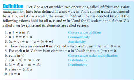
Figure 1 shows the axioms that formally define a vector space. Keep in mind that linear algebra is a huge topic in mathematics and here we’re discussing it in an informally-practical-applied-oriented manner, trying to achieve a natural feeling of how this stuff works, so I’ll keep things way more relaxed than a formal mathematical approach.

Inner Product

The inner product is an operation that takes two vectors and “spits” a scalar, i.e., a single number. In Euclidian space, this operation is defined as the sum of the product of the coordinates of the vectors, such as:

Inner Product algebraic definition

the product has an interesting geometric interpretation, it measures the angle between two vectors. Imagine now an arbitrary data distribution with p features and n inputs, entities, individuals, or constituents found in types of wine (yes, you guessed right! Another medium article with clichê dataset. Judge me, I don’t care :) ).

The infamous wine data set

Each row is a sample of one of three types of wine, described with a total of 13 features (alcohol, malic acid, etc). This data lives in an n-dimensional (13-dimensional) space, and we can compute the inner product between the columns. The angle between the vectors says a lot about their behavior, when we centralize our data (remove the mean from it) the inner product is exactly the same thing as the correlation of the variables! with pandas, we can calculate the correlation matrix as simply as df.corr(), and it gives:

correlation matrix — an ugly print

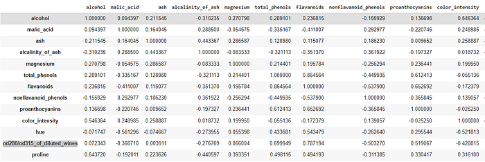
My ugly print shows the correlation matrix between the features of the wine dataset. We’ll discuss further the covariance/correlation matrix, here I just want to emphasize the geometric characteristic of the data, and that inner product = correlation of variables.

The inner product measures the angle between two vectors

It's kinda intuitive if you remember the values of the cosine of an angle. it varies from 0 to 1 (exactly like correlation), the smaller the angle, the bigger the cosine, and the closer the vectors, that is, the more similar they are, hence, the higher correlation between them. when the angle is 90 degrees (PI/2) the vectors are perpendicular, the cosine is zero, and is said that the vectors are linearly independent. if the angle is greater than 90, vectors start to point in opposite directions and the correlation becomes negative.

correlation is the cosine of the angle of two vectors (normalized dot product)

Linear Transformation — Roughly Speaking

A linear transformation is a tool to take our objects to travel (sorry, too much in the analogy yet), that is, move them from one vector space to another, BUT, it is not any kind of travel, the rules that we can apply to the objects in one space must be valid in the new one. That maybe get’s clear with the formal definition:

A linear transformation is a function L, with domain V and image W (V and W being vector spaces) satisfying:

1. L(v + u) = L(v) + L(u). (additivity property)
2. L(cv) = cL(v), for all v in V and any real number c. (homogeneity property)

if V=W, the linear transformation L: V → V is also called a linear operator.

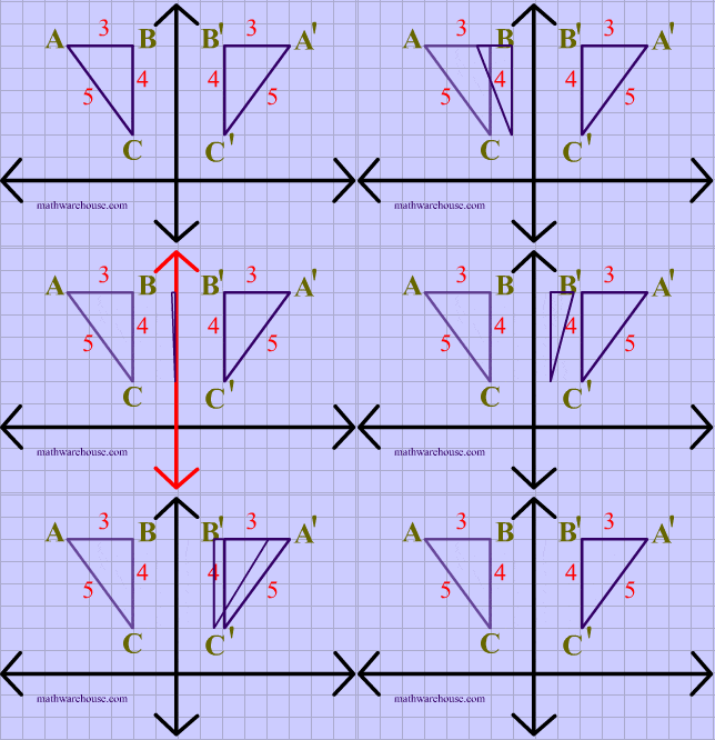
for the sake of this article, we can consider R^k as our vector space, but it's good to keep in mind that vector spaces are abstract entities, and R^k is just one kind of representation. A basic linear transformation example is a y-axis reflection:

Figure 2 — Linear Transformation illustration

It turns out that when we have well-defined vector spaces like R^n, we can represent our linear transforms through matrix operations. Suppose a linear transform L: R^n -> R^m takes vectors from an n-dimensional space to an m-dimensional space. A single matrix A (m x n) can be associated with L. This matrix will be the key to determining the eigenvectors and eigenvalues of the linear transformation, and with those, we develop the Principal Component Analysis. But first, let's just work with a simple example with some coding just for fun.

Figure 3 — meme

Let's take a simple two-dimensional distribution as above, our first toy data of this tutorial:

Figure 4 — A simple 2-dimensional distribution: Toy Data

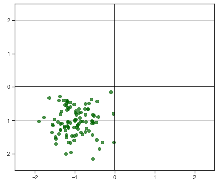
Our data points are the objects (vectors) of our vector space, R² (2-dimensional real plane), defined by their coordinates (x, y). A linear transformation that we can think of is an anti-clockwise rotation by an alpha arbitrary angle, defined by the matrix:

Figure 5 — Rotation Matrix

So, in python, we can build this matrix like this:

def rotation_matrix(alpha)
    R_alpha = np.asarray([[np.cos(alpha), -np.sin(alpha)],
                        np.sin(alpha), np.cos(alpha)]])
    return R_alpha

and, applying it to our toy data for some different angle values, we obtain the following results:

Figure 6 — applying some rotations (45, 90, and 180 degrees respectively) to our toy dataset. source: Author

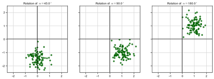
If you look closely, you can check that the “inner structure” of our data points and the distances between them are preserved while they’re being rotated. I’ve put the code to create those images in a gist if you are interested (simple stuff):

<script src=”https://gist.github.com/netofigueira/94fba3390fd65a400d9d8fa35fdada6b.js"></script>

Eigenvectors and Eigenvalues

With the concepts of vector spaces and linear transformations in mind, we can discuss the last theoretical piece to understand the PCA method, eigenvectors and eigenvalues. Take an arbitrary linear operator L and its respective matrix representation A (don’t forget that we can associate matrices to linear operators) that is, a linear transformation that takes vectors to the same vector space V. A very frequent and common question (believe me, it is) we can make is, after applying L to a vector v, the resulting vector L(v) = Av is proportional to v, i.e., Av= λv (Equation 1), where lambda is a real number.

Figure 7 illustrates such a case, it's kind of simple right?

Figure 7 — What an eigenvector looks like (in a bi-dimensional real-valued vector space)

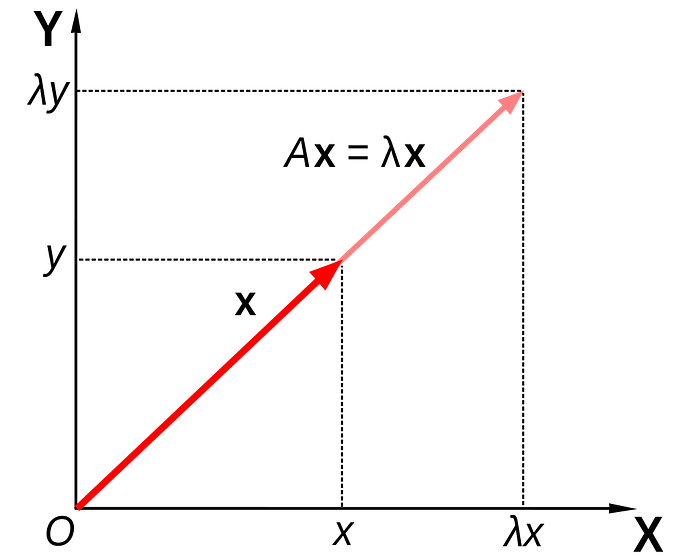
A trivial but important fact is that eigenvectors cannot be null, otherwise every number would be an eigenvalue. back to equation 1, we can rewrite it as:

(A-λI)v = 0

That's arguably the most important equation from linear algebra. The eigenvectors being always different from zero implies (A-λI) matrix must be singular, that is, its determinant is null and it cannot have an inverse matrix (why? can you answer in the comments?). from the fact that |A-λI| = 0, we calculate the respective eigenvalues λ, that's the so-called characteristic equation. After obtaining the eigenvalues, we go back to equation 1 and solve it with them to obtain the eigenvectors of A.

Covariance Matrix

Now that we are familiar with eigenvalues/vectors, let's go back to the already cited Covariance Matrix. that’s just a square matrix containing the covariance of each pair of n vectors of our space. Covariance measures the strength and direction of the relationship between two variables, mathematically:

covariance formula

covariance matrix illustration

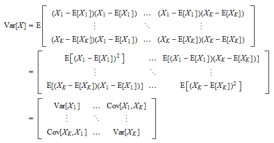
The strength is the absolute value but is not simple to interpret, it depends on the scale of the vectors, and that’s why we normalize it to obtain the correlation and correlation matrix.

If you’ve come this far, you are ready to finally dive into the PCA analysis, with all the necessary math background to understand the method. So, in Part 2 of this article, we join all the concepts discussed here together and apply them to build the PCA technique, and I promise it will be way more practical with real-world use-cases. see ya!